Summary
XLOOKUP is a powerful and incredibly versatile function within Microsoft Excel. It was introduced in 2019 as an alternative to the much-used VLOOKUP function, with the aim of simplifying searches for data within a spreadsheet. XLOOKUP offers fast and efficient lookup capabilities while also enabling users to handle more complex search criteria. One of its most impressive features is that it can look both vertically and horizontally to find data, making it easier to work with unstructured spreadsheets containing different types of data. Additionally, XLOOKUP provides options for approximate as well as exact matches, ensuring that users can quickly and easily find the information they need without having to jump through complicated hoops or resorting to manual searches. Its speed, simplicity, and flexibility make it an invaluable tool for professionals working with large datasets in any industry.
XLOOKUP Syntax
=XLOOKUP(lookup_value,lookup_array,result_array)
How to use XLOOKUP in Excel
The XLOOKUP function is designed to make finding data considerably easier by reducing the number of nested formulas required to perform lookups. To use XLOOKUP, follow these simple two steps:
- Select the cell where you want the returned result to appear and start typing the XLOOKUP formula.
- Specify which cells within your document are being searched using an array reference, along with any conditions that must be met.
Additionally, you can customize some of its base settings such as exact match mode, wildcard characters matching mode, etc., but by default XLOOKUP takes care of many automatic matching requirements.
Example of XLOOKUP
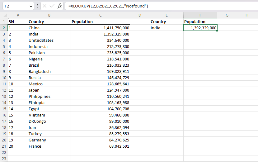
In our example, we have a list of countries in one column and the population of each country in another column. Accordingly, we want to find the population of India quickly in this table using the XLOOKUP function.
To do so, select a cell in which you want to find the population, and type the following formula:
=XLOOKUP(E2,B2:B21,C2:C21,"Notfound")
Two-Way XLOOKUP
Two-way XLOOKUP allows you to search for data in both horizontally and vertically within a table or range. To use this function, begin by selecting the cell where you would like to enter your formula. Next, enter the formula:
=XLOOKUP(lookup_value, lookup_array1, return_array1, [lookup_array2], [return_array2], [match_mode], [search_mode])
- Replace “lookup_value” with the value you would like to search for.
- Replace “lookup_array1” with the row or column containing your lookup values.
- Replace “return_array1” with the column or row from which you want to retrieve data.
- If you have additional columns or rows to include in your search range, add them as optional arguments in brackets.
- Choose your desired match mode (0 for an exact match or 1 for approximate). Also, search mode (0 for searching from left/top or 1 for searching from right/bottom).
Example of Two-Way XLOOKUP
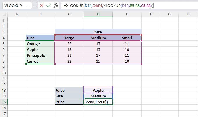
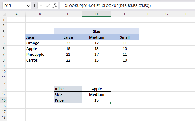
In our example, we have a list of juices in one column followed by the size of each juice and prices. As a result, we will use the XLOOKUP function to find the price for medium size Apple juice. The formula is:
=XLOOKUP(D14,C4:E4,XLOOKUP(D13,B5:B8,C5:E8))
XLOOKUP vs. VLOOKUP
XLOOKUP is a recently introduced Excel function that has gained widespread popularity for its enhanced functionality over VLOOKUP. Unlike the VLOOKUP function, XLOOKUP is capable of searching not just to the right of the lookup column, but can also search to the left and across rows. Additionally, XLOOKUP offers a superior error-handling system that makes it easier for users to create more accurate formulas. It also allows for approximate matches using wildcards and reverse lookups, which are not possible with VLOOKUP. However, both functions have their unique strengths depending on the desired outcome. While VLOOKUP may be simpler to use for basic tasks such as looking up an exact match in a table format database, XLOOKUP offers greater versatility in more complex applications where multi-criteria data searches are required. In conclusion, while they do have some overlap in their abilities, understanding when and how to best utilize each function is crucial for maximizing productivity and efficiency in Excel-based projects.
XLOOKUP vs. index and match
When it comes to sorting and retrieving data in Excel, two of the most widely used methods are XLOOKUP and INDEX MATCH. XLOOKUP is a new function introduced in Excel 365. It simplifies the process of finding information by allowing users to search for a specific value in a table or range of cells. Accordingly, it retrieves corresponding data from another column in the same table. On the other hand, INDEX MATCH is a more traditional method that involves using two formulas together. The INDEX formula returns an array of values from a specified range based on its row and column number. At the same time, the MATCH formula searches for a specific value within that range. While both methods can effectively extract data from large sets of information, XLOOKUP offers a simpler approach by eliminating multiple formulas and parameters while also handling errors better. However, INDEX MATCH provides more flexibility since it can handle complex lookup scenarios such as searching through multiple columns or ranges based on various criteria. Ultimately, the decision between these two methods depends on personal preference and specific user requirements.