VLOOKUP is a great and widely used function in Microsoft Excel that allows you to search for data within a specific table and retrieve related data from another column. The “V” letter in VLOOKUP stands for vertical, as the function searches for values vertically down a column of data. It is often used to combine data from different worksheets or workbooks, or to cross-reference data in two separate tables.
How to use VLOOKUP in Excel
To use VLOOKUP, you must specify the value you want to search for, the range of cells where the data is located, and the column number from which you want to retrieve related information. However, this tool saves time and reduces errors by automating complex calculations and reducing manual efforts on large datasets. As such, VLOOKUP is essential for many professionals that rely on Excel for their day-to-day work, including analysts, accountants, financial planners, and project managers.
What you need to perform VLOOKUP function
- The value you want to look up.
- The range in which you want to find the value and the return value.
- The number of the column within your defined range that contains the return value.
- Use FALSE or 0 for an exact match with the value you are looking for. True or 1 for an approximate match.
VLOOKUP Syntax
=VLOOKUP([value], [range], [column number], [false or true])
VLOOKUP Example
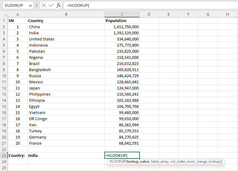
In our example, we have a list of countries in one column and the population of each country in another column. Accordingly, we want to find the population of India quickly in this table.
First, select a cell in which you want to find the population:
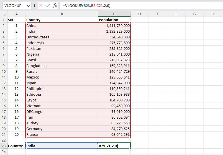
Second, select the value you want to look up, in this case it’s ‘India’ in cell B23 and start typing the following formula:
VLOOKUP(B23,B2:C21,2,0)
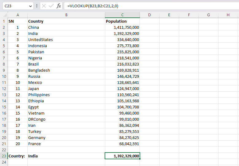
Finally, press enter to get the corresponding result from the row that contains value ‘India’ within the selected table array:
Note: It is important to ensure that your data is sorted correctly before using VLOOKUP, as this can impact its accuracy.
Additionally, you may want to consider using an IFERROR statement with your VLOOKUP formula to account for any errors or missing values. With these tips in mind, mastering VLOOKUP can greatly enhance your ability to analyze and manipulate data in Excel.
=IFERROR(VLOOKUP(B23,B2:C21,2,0),"Not found")

This will complete your formula and populate the selected cell with a result showing what column contains data corresponding to your inputs. With familiarity and practice, using VLOOKUP in Excel will become second nature for quickly and accurately finding needed data amidst complex spreadsheets.
VLOOKUP vs Index and Match in Excel
When comparing VLOOKUP and Index-Match in Excel, it’s important to understand their differences and limitations. VLOOKUP is simple to use and familiar, but it can’t lookup data located left of the lookup column, which makes it difficult to use for more complex workbooks. On the other hand, Index-Match formula offers more flexibility in terms of location with respect to the lookup value, which means we can search both horizontally and vertically. Additionally, Index-Match is faster than VLOOKUP for large datasets. Although VLOOKUP has been around for a long time and is still prevalent in many workbooks, Index-Match offers more functionality that goes beyond basic lookups. Knowing when to utilize each formula will help you handle different cases as professionally as possible.