Mastering VLOOKUP in Excel

Mastering VLOOKUP in Excel: A Comprehensive Guide with Examples

Microsoft Excel is a powerful tool used for various tasks, from basic data entry to complex financial modeling. One of the most essential functions in Excel is VLOOKUP, which stands for “Vertical Lookup.” VLOOKUP allows you to search for a specific value in a table or range and retrieve corresponding data from another column. In this article, we’ll explore the VLOOKUP formula in Excel with detailed examples to help you master this fundamental function.

Understanding the VLOOKUP Formula

The syntax for the VLOOKUP function is as follows:

				
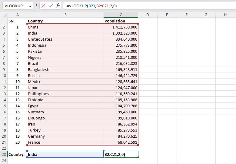
					=VLOOKUP(lookup_value, table_array, col_index_num, [range_lookup])

lookup_value: This is the value you want to find in the first column of your table or range.
table_array: The range or table where Excel should search for your lookup_value.
col_index_num: The column number from which you want to retrieve data. This is a numeric value, with 1 representing the first column in the table_array.
[range_lookup]: An optional argument that specifies whether you want an exact match (FALSE or 0) or an approximate match (TRUE or 1). If omitted, Excel assumes an approximate match.

Using VLOOKUP for Exact Matches

Let’s start with a straightforward example of using VLOOKUP formula for exact matches. Suppose you have a table of products and their prices, and you want to find the price of a specific product.

Table: Product Prices

Product	Price
Apple	1.00
Banana	0.75
Orange	1.25
Grape	1.50
Watermelon	3.00

To find the price of an apple, you would use the following formula:

				
					=VLOOKUP("Apple", A2:B6, 2, FALSE)

Here’s what each part of the formula does:

lookup_value: “Apple” – The product you’re looking for.
table_array: A2:B6 – The table where Excel should search for “Apple.”
col_index_num: 2 – The price column is the second column in the table_array.
range_lookup: FALSE – Indicates that you want an exact match.

The formula would return the value 1.00, which is the price of an apple.

Using VLOOKUP for Approximate Matches

VLOOKUP is also commonly used to perform approximate matches, especially when dealing with large datasets. Let’s consider an example where you have a table of grades and corresponding letter grades.

Table: Grade Scale

Grade	Letter
90-100	A
80-89	B
70-79	C
60-69	D
0-59	F

Now, if you want to determine the letter grade for a score of 85, you would use VLOOKUP with an approximate match:

				
					=VLOOKUP(85, E2:F6, 2, TRUE)

In this case, the formula works as follows:

lookup_value: 85 – The score you’re looking up.
table_array: E2:F6 – The table containing the grade scale.
col_index_num: 2 – The second column (Letter grades) in the table_array.
range_lookup: TRUE – Specifies an approximate match.

The formula would return “B” because 85 falls within the range of 80-89, which corresponds to a letter grade of “B.”

Handling Errors with VLOOKUP

When using VLOOKUP, it’s essential to account for potential errors, especially when the lookup_value is not found in the table. You can use the IFERROR function to display a custom message instead of the default #N/A error.

For example, if you’re looking up a product called “Mango” that doesn’t exist in the Product Prices table, you can use this formula:

				
					=IFERROR(VLOOKUP("Mango", A2:B6, 2, FALSE), "Product not found")

This formula will display “Product not found” instead of #N/A if “Mango” is not in the table.

Conclusion

VLOOKUP is a powerful Excel function that allows you to search for specific values in tables or ranges and retrieve corresponding data. Whether you need to perform exact matches or approximate matches, VLOOKUP is a valuable tool for data analysis and reporting. With the examples provided in this article, you should now have a solid understanding of how to use VLOOKUP effectively in your Excel spreadsheets.

Mastering VLOOKUP in Excel