Microsoft Excel PivotTable is a powerful data analysis tool that allows you to summarize, group, and analyze large amounts of data from different sources. With PivotTable, you can quickly organize and analyze complex data sets into meaningful reports or charts without having to manually aggregate the data themselves. Moreover, it allows you to filter, sort, and explore data in a dynamic way to make more informed decisions. Additionally, PivotTable works seamlessly with other Excel features such as Charts, Slicers, and Power Query. Overall, Microsoft Excel PivotTable is an essential tool for any professional or organization looking to make better use of their data.
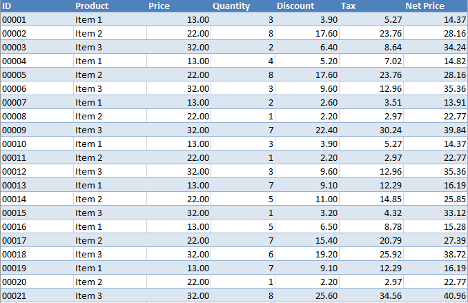
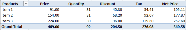
Below Tables show the difference between Row Data and a Pivot Table:
A. Example of a normal Excel Row Data
B. Example of an Excel PivotTable
How to create Excel PivotTable
To create an Excel Pivot Table, follow the below steps:
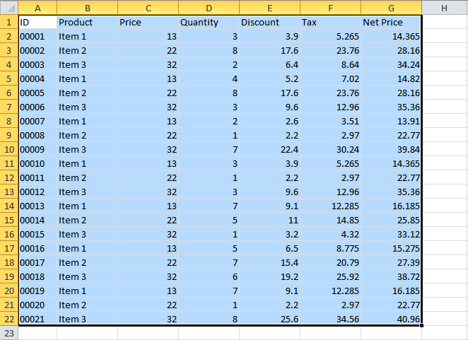
- Highlight the original row data and press Ctrl + t to convert it to a normal table.
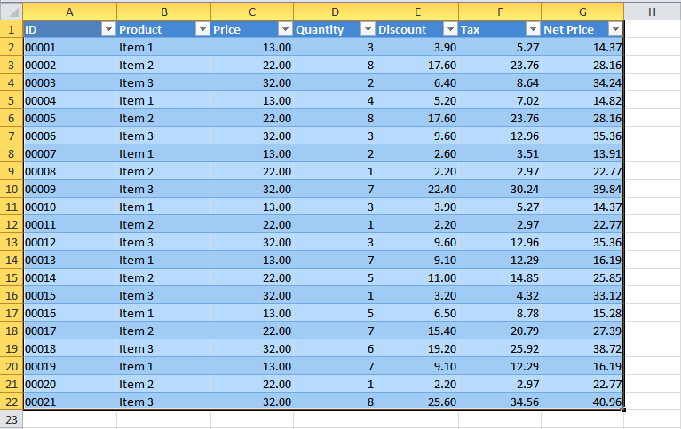
The range will be transformed into a table:
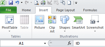
2. Click on the Insert tab, then click on the Tables group, and finally click on the PivotTable icon.
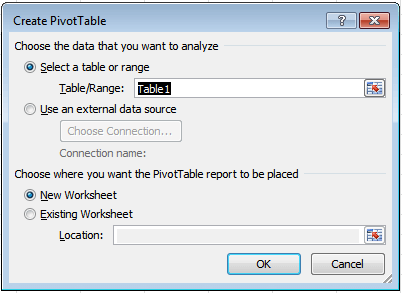
3. The following dialog box will appear. Select where you want the PivotTable report to be placed and click OK.
4. The PivotTable Fields panel will appear on the right side of the worksheet. All you need is to drag the fields between the areas:
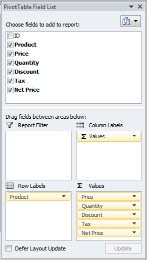
Upon selecting fields from the list, you will notice that the pivot table updates itself automatically. You can continue till you get the perfect summary out of the original row data.
In addition, you can sort, filter, and update the pivot table like you would with normal tables. Lastly, if you update the row data, then you will need to refresh the pivot table under Data Panel.
More information about Microsoft Excel PivotTable